Lecture 2.2: Interferometers and the Bloch Sphere

Review of Last Lecture¶

In Lecture 2.1, we established the key ideas about waves and interference:

• Traveling waves in complex form: $E(x,t) = E_0 e^{i(kx - \omega t)}$

• Intensity is the magnitude squared: $I \propto |E|^2$

• Interference comes from adding amplitudes before squaring:

• For two sources with phases $\phi_1$ and $\phi_2$:

• Only the relative phase matters — the intensity depends on $\phi_1 - \phi_2$, not on the individual phases.

Today we’ll explore two important interferometers: the Michelson interferometer (historically crucial for physics) and the Mach-Zehnder interferometer (conceptually cleaner for quantum computing). Then we’ll develop the Bloch sphere as a way to visualize qubit states.

iClicker: Review Question¶

Two waves interfere with intensity $I = |e^{i \phi_1} + e^{i \phi_2} |^2$. If $\Delta\phi = \pi$, the interference is:

• (A) Constructive ($I = 4$)

• (B) Destructive ($I = 0$) ✓

• (C) Partially constructive ($I = 2$)

• (D) Depends on the wavelength

The Michelson Interferometer¶

Before we dive into the Mach-Zehnder interferometer, let’s discuss its historically important cousin: the Michelson interferometer.

The Setup¶

Components:

• BS: A 50/50 beam splitter at 45° to the incoming beam

• M1, M2: Mirrors that reflect light back toward the beam splitter

• Arm 1 and Arm 2: The two paths, with lengths $L_1$ and $L_2$

• Detector: Measures the output intensity

The key difference from the Mach-Zehnder is that light travels back and forth in each arm, so the total path length in arm $j$ is $2L_j$.

The Calculation¶

Following the same approach as before, light entering the interferometer is split at the beam splitter. After traveling to the mirrors and back:

where $\phi_j = 2kL_j = \frac{4\pi L_j}{\lambda}$ (note the factor of 2 from the round trip).

When the beams recombine at the beam splitter, the detected intensity is:

where $\Delta\phi = \phi_1 - \phi_2 = \frac{4\pi}{\lambda}(L_1 - L_2)$.

The interferometer is maximally sensitive when $\Delta\phi \approx \pi/2$, where small changes in path length cause large changes in intensity.

Historical Significance: The Michelson-Morley Experiment¶

In 1887, Albert Michelson and Edward Morley performed one of the most important experiments in the history of physics using this interferometer.

The question they asked: Does light travel through a medium called the “luminiferous ether”?

In the 19th century, physicists believed that light waves, like sound waves, must propagate through some medium. They called this hypothetical medium the “ether” and assumed it filled all of space. If Earth moves through this ether, then the speed of light should be different in different directions—faster when moving with the ether, slower when moving against it.

The experiment: Michelson and Morley oriented their interferometer so that one arm pointed in the direction of Earth’s motion through space (about 30 km/s around the Sun), and the other arm was perpendicular. If light traveled through an ether, the round-trip times in the two arms would differ slightly, causing a phase shift. By rotating the entire apparatus, they expected to see the interference pattern shift.

The result: Nothing. No matter how they oriented the interferometer or what time of year they measured, they found no difference in the speed of light in different directions. The expected fringe shift was about 0.4 fringes; they observed less than 0.01 fringes.

The implication: The speed of light is the same in all directions, regardless of the motion of the observer. This null result was deeply puzzling at the time, but it became one of the key experimental foundations for Einstein’s special theory of relativity (1905), which postulates that the speed of light is constant in all inertial reference frames.

Modern Application: LIGO and Gravitational Waves¶

The same basic principle—measuring tiny path length differences via interference—is used today in the most sensitive displacement measurements ever made: the Laser Interferometer Gravitational-Wave Observatory (LIGO).

The setup: LIGO is essentially a giant Michelson interferometer with arms 4 km long. Laser light travels back and forth in each arm about 280 times (using Fabry-Pérot cavities), giving an effective path length of over 1000 km.

The sensitivity: When a gravitational wave passes through LIGO, it stretches space in one direction while compressing it in the perpendicular direction. This causes a differential change in the arm lengths. LIGO can detect changes in arm length of:

To put this in perspective:

• A hydrogen atom is about 10^-10 m

• A proton is about 10^-15 m

• LIGO measures displacements 1000 times smaller than a proton!

How is this possible? The key is that interferometry measures path length relative to the wavelength $\lambda \approx 1 \,\mu\text{m}$. A phase shift of $\Delta\phi = 0.001$ radians corresponds to a path length change of:

By using sophisticated techniques (high laser power, multiple bounces, quantum squeezing of light), LIGO pushes this sensitivity to extraordinary levels. In 2015, LIGO made the first direct detection of gravitational waves from merging black holes—a discovery that earned the 2017 Nobel Prize in Physics.

The Mach-Zehnder Interferometer¶

The Mach-Zehnder interferometer (MZI) is conceptually cleaner than the Michelson because light travels through each arm only once, and there are two distinct output ports.

The Setup¶

Components:

• BS1: First 50/50 beam splitter — splits incoming light equally into two arms

• Arm 1 and Arm 2: The two paths, with lengths $L_1$ and $L_2$

• M1, M2: Mirrors that redirect the beams toward the second beam splitter

• BS2: Second 50/50 beam splitter — recombines the two beams

• D1, D2: Two detectors that measure the output intensity

The Beam Splitter: Why the Phase Shift?¶

Before we calculate, let’s understand a crucial property of beam splitters: reflection from one side must pick up a π phase shift relative to reflection from the other side.

Why? Energy conservation.

Consider what would happen if there were no phase shift. With equal amplitudes $a$ entering from each input port, the outputs would be:

The total output power would be $|E_{out1}|^2 + |E_{out2}|^2 = 4|a|^2$, but the input power is only $2|a|^2$. We’ve created energy from nothing!

With the phase shift, if one reflection picks up a minus sign:

Now the total output power is $2|a|^2$, which equals the input. Energy is conserved.

The physical origin of this phase shift depends on the type of beam splitter. For a dielectric beam splitter, it comes from the boundary conditions for electromagnetic waves: reflection from the high-index side picks up no phase shift, while reflection from the low-index side picks up a π phase shift.

Calculation Using Wave Amplitudes¶

Let’s analyze the MZI using the complex amplitude formalism.

Step 1: Input and first beam splitter

An incident wave arrives at BS1:

At the beam splitter (position $x = 0$), the wave is split equally:

The factor of $1/\sqrt{2}$ ensures intensity conservation: $|E_{arm1}|^2 + |E_{arm2}|^2 = |E_0|^2$.

Step 2: Phase accumulation

After traveling distance $L_j$ in arm $j$:

where $\phi_j = kL_j = \frac{2\pi}{\lambda} L_j$.

Step 3: Second beam splitter and detection

At BS2, including the phase shift from reflection:

• Detector D1 receives the sum of the two amplitudes

• Detector D2 receives the difference (one path has the π phase shift)

Step 4: Calculate intensities

Using $|e^{i\phi_1} + e^{i\phi_2}|^2 = 2(1 + \cos(\phi_1 - \phi_2))$ and normalizing:

where $\Delta\phi = \phi_1 - \phi_2 = k(L_1 - L_2)$.

Key Results¶

Important observations:

1. Conservation of energy: $I_{D1} + I_{D2} = 1$. All the light goes somewhere!

2. Complementary outputs: When D1 is bright, D2 is dark, and vice versa.

3. Only the phase difference matters: The intensities depend on $\Delta\phi = \phi_1 - \phi_2$, not on $\phi_1$ and $\phi_2$ individually.

Global Phase Doesn’t Matter¶

Let’s verify explicitly that only relative phase matters.

Adding a common phase $\gamma$ to both arms:

The intensity:

The global phase $e^{i\gamma}$ has magnitude 1, so it drops out!

The MZI as a Quantum Circuit¶

Now let’s rewrite the calculation using matrix notation. This reveals that the MZI is mathematically identical to a quantum computing circuit.

State Vector Notation¶

Instead of tracking separate amplitudes, we combine them into a state vector:

where $c_1$ is the amplitude in arm 1 (path $|0\rangle$) and $c_2$ is the amplitude in arm 2 (path $|1\rangle$).

The input light enters arm 1 only:

The Hadamard Matrix (Beam Splitter)¶

A 50/50 beam splitter is represented by the Hadamard matrix:

Notice the minus sign in the (2,2) position—this is the π phase shift we discussed!

Let’s verify this does what we expect:

Equal amplitude $1/\sqrt{2}$ in each arm, as expected.

The Phase Gate¶

The relative phase between arms is represented by:

This applies phase $\phi$ to the $|1\rangle$ component while leaving $|0\rangle$ unchanged.

The Full Calculation¶

The MZI corresponds to:

Step 1: Apply first Hadamard

Step 2: Apply phase gate

Step 3: Apply second Hadamard

Detection probabilities:

This matches our wave calculation exactly!

The Quantum Circuit Diagram¶

Measurement as Projection¶

What does “measurement” mean mathematically? When we measure in the $\{|0\rangle, |1\rangle\}$ basis, we project the state onto one of these basis vectors.

For a state $|\psi\rangle = c_0|0\rangle + c_1|1\rangle$:

• Probability of measuring $|0\rangle$: $P(0) = |\langle 0|\psi\rangle|^2 = |c_0|^2$

• Probability of measuring $|1\rangle$: $P(1) = |\langle 1|\psi\rangle|^2 = |c_1|^2$

The detectors D1 and D2 in our interferometer are doing exactly this: D1 measures whether the photon is in the $|0\rangle$ state (output port 1), and D2 measures whether it’s in $|1\rangle$ (output port 2).

This is a general principle: measurement collapses the quantum state onto one of the measurement basis states, with probability given by the squared magnitude of the amplitude.

iClicker: Beam Splitter with Two Inputs¶

A beam splitter has two inputs: amplitude 1 enters from the top, and amplitude $e^{i\theta}$ enters from the side. The Hadamard matrix gives the outputs. What value of $\theta$ gives equal power in both outputs?

Setup: Input state is $|\psi_{in}\rangle = \begin{pmatrix} 1 \\ e^{i\theta} \end{pmatrix}$

Output: $|\psi_{out}\rangle = H|\psi_{in}\rangle = \frac{1}{\sqrt{2}}\begin{pmatrix} 1 + e^{i\theta} \\ 1 - e^{i\theta} \end{pmatrix}$

• (A) $\theta = 0$

• (B) $\theta = \pi/2$ ✓

• (C) $\theta = \pi$

• (D) $\theta = 3\pi/4$

Solution: For equal power, we need $|1 + e^{i\theta}|^2 = |1 - e^{i\theta}|^2$.

Using $|1 + e^{i\theta}|^2 = 2(1 + \cos\theta)$ and $|1 - e^{i\theta}|^2 = 2(1 - \cos\theta)$:

Equal power requires $1 + \cos\theta = 1 - \cos\theta$, which means $\cos\theta = 0$.

This gives $\theta = \pi/2$ or $\theta = 3\pi/2$.

The Bloch Sphere¶

We’ve seen that a qubit state can be written as:

How do we visualize this?

Counting Degrees of Freedom¶

Start: Two complex numbers = 4 real parameters

Constraint 1: Normalization $|c_0|^2 + |c_1|^2 = 1$ removes one parameter: 3 real parameters

Constraint 2: Global phase is unobservable We can make $c_0$ real and non-negative: 2 real parameters

The Bloch Parametrization¶

With these constraints:

where:

• $\theta \in [0, \pi]$ is the polar angle (from the north pole)

• $\phi \in [0, 2\pi)$ is the azimuthal angle (around the equator)

Every qubit state corresponds to a point on the unit sphere: the Bloch sphere.

Key Points on the Bloch Sphere¶

Orthogonal States are Antipodal¶

Orthogonal quantum states are on opposite sides of the Bloch sphere.

• $|0\rangle$ (north pole) and $|1\rangle$ (south pole): orthogonal ✓

• $|+\rangle$ (+x) and $|-\rangle$ (−x): orthogonal ✓

• $|+i\rangle$ (+y) and $|-i\rangle$ (−y): orthogonal ✓

This is why we use $\theta/2$ in the parametrization—it makes orthogonal states antipodal.

Gates as Rotations on the Bloch Sphere¶

Here’s a beautiful geometric picture: quantum gates correspond to rotations of the Bloch sphere.

The phase gate $P(\phi)$ rotates the Bloch sphere around the z-axis by angle $\phi$:

• States on the z-axis ($|0\rangle$ and $|1\rangle$) are unchanged

• States on the equator rotate around the equator

The Hadamard gate $H$ is a rotation by $\pi$ around an axis halfway between x and z (the direction $(1, 0, 1)/\sqrt{2}$):

• It swaps the z-axis and x-axis

• $|0\rangle \to |+\rangle$ and $|+\rangle \to |0\rangle$

iClicker Questions¶

iClicker 1: A state has Bloch coordinates $\theta = \pi/2$, $\phi = \pi/2$. What is the state?

• (A) $|0\rangle$

• (B) $|1\rangle$

• (C) $\frac{1}{\sqrt{2}}(|0\rangle + |1\rangle)$

• (D) $\frac{1}{\sqrt{2}}(|0\rangle + i|1\rangle)$ ✓

Solution: With $\theta = \pi/2$: $\cos(\pi/4) = \sin(\pi/4) = 1/\sqrt{2}$. With $\phi = \pi/2$: $e^{i\pi/2} = i$. So $|\psi\rangle = \frac{1}{\sqrt{2}}(|0\rangle + i|1\rangle) = |+i\rangle$.

iClicker 2: I start with $|+\rangle = \frac{1}{\sqrt{2}}(|0\rangle + |1\rangle)$ on the +x axis and apply the phase gate $P(\pi) = \begin{pmatrix} 1 & 0 \\ 0 & -1 \end{pmatrix}$. Where do I end up on the Bloch sphere?

• (A) +x axis (same place)

• (B) −x axis ✓

• (C) +y axis

• (D) North pole

Solution:

The phase gate rotated us by $\pi$ around the z-axis, taking +x to −x.

Visualizing the MZI on the Bloch Sphere¶

The MZI sequence: $|0\rangle \xrightarrow{H} \xrightarrow{P(\phi)} \xrightarrow{H}$

1. Start: $|0\rangle$ at north pole

2. After H: $|+\rangle$ on +x axis (equator)

3. After P(φ): Rotate around z-axis by φ, staying on equator

4. After second H: Final position depends on φ

Visualizing States with Qiskit¶

Qiskit is a Python library for quantum computing that includes tools for visualizing quantum states on the Bloch sphere.

Installation¶

Run this once to install Qiskit:

# Uncomment the line below and run once to install, then comment it out
# !pip install qiskit

Basic Bloch Sphere Visualization¶

import numpy as np
from qiskit.quantum_info import Statevector
from qiskit.visualization import plot_bloch_multivector

def bloch_state(theta, phi):
    """
    Create qubit state: cos(theta/2)|0> + e^(i*phi)*sin(theta/2)|1>
    
    Parameters:
        theta: polar angle from north pole (0 to pi)
        phi: azimuthal angle around equator (0 to 2*pi)
    
    Returns:
        Qiskit Statevector object
    """
    c0 = np.cos(theta / 2)
    c1 = np.exp(1j * phi) * np.sin(theta / 2)
    return Statevector([c0, c1])

# Example: Plot the |+i⟩ state (theta = pi/2, phi = pi/2)
state = bloch_state(np.pi/2, np.pi/2)
plot_bloch_multivector(state)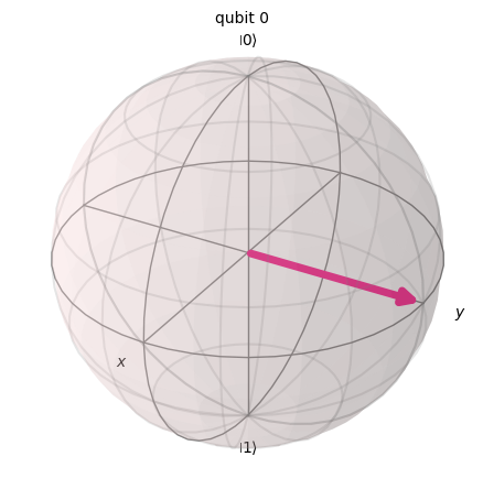

Plotting the Six Cardinal States¶

import numpy as np
from qiskit.quantum_info import Statevector
from qiskit.visualization import plot_bloch_multivector
import matplotlib.pyplot as plt

# Define the six cardinal states
states = {
    '|0⟩': Statevector([1, 0]),
    '|1⟩': Statevector([0, 1]),
    '|+⟩': Statevector([1, 1]) / np.sqrt(2),
    '|−⟩': Statevector([1, -1]) / np.sqrt(2),
    '|+i⟩': Statevector([1, 1j]) / np.sqrt(2),
    '|−i⟩': Statevector([1, -1j]) / np.sqrt(2),
}

# Plot each state
for name, state in states.items():
    print(f"\n{name}:")
    display(plot_bloch_multivector(state))

Visualizing the MZI Sequence¶

import numpy as np
from qiskit.quantum_info import Statevector, Operator
from qiskit.visualization import plot_bloch_multivector

# Define gates
H = Operator([[1, 1], [1, -1]]) / np.sqrt(2)  # Hadamard

def phase_gate(phi):
    """Phase gate P(phi) = diag(1, e^(i*phi))"""
    return Operator([[1, 0], [0, np.exp(1j * phi)]])

# MZI with phase = pi/2
phi = np.pi / 2

psi = Statevector([1, 0])       # Start at |0⟩
print("Initial |0⟩:")
display(plot_bloch_multivector(psi))

psi = psi.evolve(H)             # After first Hadamard
print("After H:")
display(plot_bloch_multivector(psi))

psi = psi.evolve(phase_gate(phi))  # After phase gate
print(f"After P({phi:.2f}):")
display(plot_bloch_multivector(psi))

psi = psi.evolve(H)             # After second Hadamard  
print("Final state:")
display(plot_bloch_multivector(psi))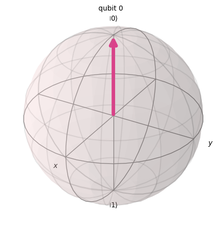

Homework: Interferometers and the Bloch Sphere¶

This homework is designed to be completed in Python. You’ll use NumPy for linear algebra and Qiskit for visualization.

Setup¶

First, install the required packages if you haven’t already:

# Uncomment and run once to install, then comment out
# !pip install qiskit numpy matplotlib

Import the libraries you’ll need:

import numpy as np
from qiskit.quantum_info import Statevector
from qiskit.visualization import plot_bloch_multivector
import matplotlib.pyplot as plt

Problem 1: Bloch Sphere Visualization¶

The six cardinal states on the Bloch sphere are fundamental reference points for understanding qubit states.

Part (a): Create a State Table¶

Complete the following table by filling in the state vector components $c_0$ and $c_1$ for each state, where $|\psi\rangle = c_0|0\rangle + c_1|1\rangle$.

Part (b): Create States in Python¶

Write Python code to create each of the six cardinal states as Qiskit Statevector objects. Store them in a dictionary called cardinal_states with keys '|0⟩', '|1⟩', '|+⟩', '|−⟩', '|+i⟩', '|−i⟩'.

# Your code here
cardinal_states = {
    '|0⟩': # ...,
    '|1⟩': # ...,
    # ... complete for all six states
}

Part (c): Visualize All Six States¶

Write a loop that plots each of the six cardinal states on the Bloch sphere. Include a title for each plot indicating which state is being displayed.

Problem 2: Quantum Gates¶

Part (a): Define the Hadamard Gate¶

The Hadamard gate is:

Define this as a NumPy array. Verify that $H$ is unitary by showing that $H H^\dagger = I$ (the identity matrix). Later we will learn that this means that energy is conserved on the output.

Part (b): Define the Phase Gate Function¶

The phase gate with parameter $\phi$ is:

Write a function phase_gate(phi) that returns this matrix as a NumPy array:

def phase_gate(phi):
    """
    Returns the phase gate P(phi) as a 2x2 numpy array.
    
    Parameters:
        phi: phase angle in radians
        
    Returns:
        2x2 numpy array representing P(phi)
    """
    # Your code here

Test your function by verifying that:

• $P(0) = I$ (identity matrix)

• $P(\pi)$ has a -1 in the bottom-right corner

Part (c): Apply Gates to States¶

Using your definitions of $H$ and phase_gate():

1. Compute $H|0\rangle$ and verify it equals $|+\rangle$

2. Compute $P(\pi)|+\rangle$ and verify it equals $|-\rangle$

3. Compute $H|+\rangle$ and verify it equals $|0\rangle$

# Define |0⟩
ket_0 = np.array([1, 0])

# 1. Compute H|0⟩
result1 = # ...
print("H|0⟩ =", result1)

# 2. Compute P(π)|+⟩
# ...

# 3. Compute H|+⟩
# ...

Problem 3: Mach-Zehnder Interferometer Simulation¶

In this problem, you’ll simulate the complete Mach-Zehnder interferometer and reproduce the interference pattern.

Part (a): MZI Output Calculation¶

The MZI applies the sequence $H \to P(\phi) \to H$ to an input state $|0\rangle$.

Write a function mzi_output(phi) that takes a phase $\phi$ and returns the output state vector:

def mzi_output(phi):
    """
    Compute the output state of a Mach-Zehnder interferometer.
    
    The MZI applies H -> P(phi) -> H to |0⟩.
    
    Parameters:
        phi: relative phase between the two arms (radians)
        
    Returns:
        Output state as a numpy array [c0, c1]
    """
    # Your code here

Test your function:

• mzi_output(0) should return (approximately) $|0\rangle = [1, 0]$

• mzi_output(np.pi) should return (approximately) $|1\rangle = [0, 1]$

Part (b): Calculate Detection Probabilities¶

The probability of detecting the photon at detector D1 (output port 0) is $P_{D1} = |c_0|^2$, and at D2 is $P_{D2} = |c_1|^2$.

Write a function detection_probabilities(phi) that returns both probabilities:

def detection_probabilities(phi):
    """
    Compute detection probabilities for the MZI.
    
    Parameters:
        phi: relative phase between the two arms (radians)
        
    Returns:
        Tuple (P_D1, P_D2) of detection probabilities
    """
    # Your code here

Verify that $P_{D1} + P_{D2} = 1$ for several values of $\phi$.

Part (c): Plot the Interference Pattern¶

Create a plot showing $P_{D1}$ and $P_{D2}$ as functions of $\phi$ from 0 to $4\pi$.

Your plot should:

• Show both $P_{D1}(\phi)$ (perhaps in blue) and $P_{D2}(\phi)$ (perhaps in red) on the same axes

• Have proper axis labels: “$\phi$ (radians)” and “Detection Probability”

• Include a legend identifying each curve

• Have a title: “Mach-Zehnder Interferometer Output”

# Create array of phi values
phi_values = np.linspace(0, 4 * np.pi, 200)

# Calculate probabilities for each phi
P_D1 = # ...
P_D2 = # ...

# Create the plot
plt.figure(figsize=(10, 6))
# Your plotting code here

plt.show()